import numpy as np
import sympy
import matplotlib.pyplot as plt

from qrate import solvers
from pmm_tools import models, optimization, utils
from second_quantization import hilbert_space

from IPython.display import display

import logging

logging.getLogger("matplotlib.font_manager").disabled = True
Transport in a minimal Kitaev chain
In this example, we will simulate a minimal Kitaev chain made up of two normal quantum dots connected by a superconducting dot. We will use three tiny python packages to facilitate the simulation:
-
second_quantization: for finding the numerical representation of a second quantization Hamiltonian -
pmm_tools: for writing down the Hamiltonian and finding the sweet spot of the chain -
qrate: for calculating the transport properties
Define the Hamiltonian
We will use the pmm_tools package to define the Hamiltonian of the system
and the parameters of the system.
This package allows us to write a position dependent Hamiltonian in a very simple way.
We provide the length of the chain and the parameters of the system.
The parameters are defined as a dictionary, where the keys are the names of the parameters and the values are lists of sympy symbols corresponding to each site.
length = 3
mu_L, mu_M, mu_R = sympy.symbols("mu_L mu_M mu_R", real=True, positive=True)
U, E_Z, Delta, t, theta = sympy.symbols("U E_Z Delta t theta", real=True, positive=True)

_parameters = {
    "mu": [mu_L, mu_M, mu_R],
    "U": [U, 0, U],
    "E_z": [E_Z, 0, E_Z],
    "Delta": [sympy.S.Zero, Delta, sympy.S.Zero],
    "t_n": t * sympy.cos(theta / 2),
    "t_so": t * sympy.sin(theta / 2),
}
_parameters, hamiltonian, fermions = models.dot_abs_chain(length, _parameters)
terms = hilbert_space.to_matrix(hamiltonian, fermions, sparse=False)
f_hamiltonian = hilbert_space.make_dict_callable(terms)
parity_operator = hilbert_space.parity_operator(fermions, sparse=False)
display(hamiltonian)
$\displaystyle \Delta {c_{1\downarrow}} {c_{1\uparrow}} + \Delta {{c_{1\uparrow}}^\dagger} {{c_{1\downarrow}}^\dagger} + U {{c_{0\uparrow}}^\dagger} {c_{0\uparrow}} {{c_{0\downarrow}}^\dagger} {c_{0\downarrow}} + U {{c_{2\uparrow}}^\dagger} {c_{2\uparrow}} {{c_{2\downarrow}}^\dagger} {c_{2\downarrow}} + \mu_{M} {{c_{1\downarrow}}^\dagger} {c_{1\downarrow}} + \mu_{M} {{c_{1\uparrow}}^\dagger} {c_{1\uparrow}} + t \sin{\left(\frac{\theta}{2} \right)} \left({{c_{0\downarrow}}^\dagger} {c_{1\uparrow}} + {{c_{1\uparrow}}^\dagger} {c_{0\downarrow}}\right) - t \sin{\left(\frac{\theta}{2} \right)} \left({{c_{0\uparrow}}^\dagger} {c_{1\downarrow}} + {{c_{1\downarrow}}^\dagger} {c_{0\uparrow}}\right) + t \sin{\left(\frac{\theta}{2} \right)} \left({{c_{1\downarrow}}^\dagger} {c_{2\uparrow}} + {{c_{2\uparrow}}^\dagger} {c_{1\downarrow}}\right) - t \sin{\left(\frac{\theta}{2} \right)} \left({{c_{1\uparrow}}^\dagger} {c_{2\downarrow}} + {{c_{2\downarrow}}^\dagger} {c_{1\uparrow}}\right) + t \cos{\left(\frac{\theta}{2} \right)} \left({{c_{0\downarrow}}^\dagger} {c_{1\downarrow}} + {{c_{1\downarrow}}^\dagger} {c_{0\downarrow}}\right) + t \cos{\left(\frac{\theta}{2} \right)} \left({{c_{0\uparrow}}^\dagger} {c_{1\uparrow}} + {{c_{1\uparrow}}^\dagger} {c_{0\uparrow}}\right) + t \cos{\left(\frac{\theta}{2} \right)} \left({{c_{1\downarrow}}^\dagger} {c_{2\downarrow}} + {{c_{2\downarrow}}^\dagger} {c_{1\downarrow}}\right) + t \cos{\left(\frac{\theta}{2} \right)} \left({{c_{1\uparrow}}^\dagger} {c_{2\uparrow}} + {{c_{2\uparrow}}^\dagger} {c_{1\uparrow}}\right) + \left(- E_{Z} + \mu_{L}\right) {{c_{0\downarrow}}^\dagger} {c_{0\downarrow}} + \left(- E_{Z} + \mu_{R}\right) {{c_{2\downarrow}}^\dagger} {c_{2\downarrow}} + \left(E_{Z} + \mu_{L}\right) {{c_{0\uparrow}}^\dagger} {c_{0\uparrow}} + \left(E_{Z} + \mu_{R}\right) {{c_{2\uparrow}}^\dagger} {c_{2\uparrow}}$
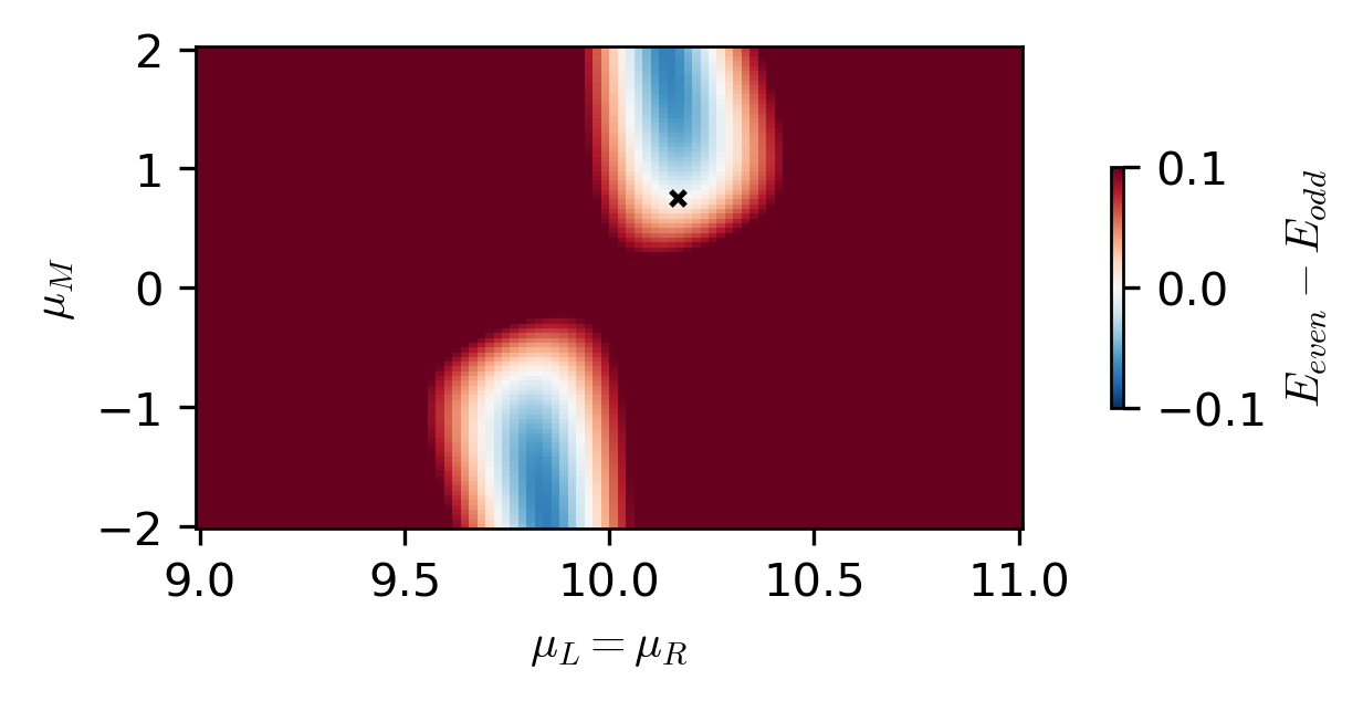
Find the sweet spot
The sweet spot is the point in the parameter space where the energy difference between the even and odd ground states is minimized.
We will use the pmm_tools package to find the sweet spot.
We will define a function that calculates the energy difference between the even and odd ground states.
This function will take the parameters of the system as input and return the energy difference.
We will then use the pmm_tools.optimization module to find the sweet spot
by minimizing the energy difference function.
parameters = {
    "U": 100,
    "E_Z": 10,
    "t": 0.6,
    "theta": 0.2 * np.pi,
    "Delta": 1,
}

# Define optimization functions


def f_energy(parity_operator=parity_operator, **parameters):
    """
    Calculate the energy difference between the even and odd ground states.
    """
    mat = f_hamiltonian(**parameters)
    evals, _ = utils.fermionic_eigsh(mat, parity=parity_operator)
    return evals[0][0] - evals[1][0]


energy_diff = optimization.wrapper_energy(parameters, f_energy)
initial_guess = (parameters["E_Z"], parameters["E_Z"], parameters["Delta"] / 2)
sweet_spot = optimization.find_sweetspot(energy_diff, initial_guess)

_mu_L = sweet_spot.x[0]
_mu_R = sweet_spot.x[1]
_mu_M = sweet_spot.x[2]
# Compute the phase diagram to validate that the sweet spot is correct
mus = np.linspace(-1, 1, 100) + parameters["E_Z"]
mus_ABS = np.linspace(-2, 2, 101)

energy_results = np.array(
    [
        f_energy(mu_L=mu, mu_M=mu_ABS, mu_R=mu, **parameters)
        for mu in mus
        for mu_ABS in mus_ABS
    ]
)
energy_results = energy_results.reshape(len(mus), len(mus_ABS))
fig, ax = plt.subplots(figsize=(4, 2))
c = ax.pcolormesh(
    mus, mus_ABS, energy_results.T, shading="auto", vmin=-1e-1, vmax=1e-1, cmap="RdBu_r"
)
ax.scatter(_mu_L, _mu_M, c="black", marker="x", s=10, label="minimization result")
ax.set_xlabel(r"$\mu_L = \mu_R$")
ax.set_ylabel(r"$\mu_M$")
cbar = fig.colorbar(c, ax=ax, location="right", shrink=0.5)
cbar.set_label(r"$E_{even} - E_{odd}$")
Define the leads
We will define the leads of the system as a list of FermionOp times the coupling strength.
The leads are defined as a list of FermionOp objects, where each FermionOp represents the site where the lead is connected to the system.
We consider two leads connected to the first and last sites of the chain.
gamma_0, gamma_2 = sympy.symbols("Gamma_0 Gamma_2", real=True, positive=True)
leads = [gamma_0 * (fermions[0] + fermions[1]), gamma_2 * (fermions[4] + fermions[5])]
for lead in leads:
    display(lead)
$\displaystyle \Gamma_{0} \left({c_{0\downarrow}} + {c_{0\uparrow}}\right)$
$\displaystyle \Gamma_{2} \left({c_{2\downarrow}} + {c_{2\uparrow}}\right)$
Calculate the current
We will use the qrate.solvers module to calculate the current through the system.
The current_solver function takes the following arguments:
-
f_hamiltonian: a callable function that returns the Hamiltonian of the system -
f_leads: a list of callable functions that return the leads of the system -
parameters: a dictionary of parameters of the system -
lead_parameters: a dictionary of parameters of the leads -
kbT: the thermal energy of the system, default is 0.01
To create the callable functions, we will use the hilbert_space.to_matrix function to convert the Hamiltonian and leads to a matrix representation.
# Define the callables
hamiltonian_dict = hilbert_space.to_matrix(hamiltonian, operators=fermions, sparse=False)
f_hamiltonian = hilbert_space.make_dict_callable(hamiltonian_dict)

lead_dicts = [
    hilbert_space.to_matrix(lead, operators=fermions, sparse=False) for lead in leads
]
f_leads = [hilbert_space.make_dict_callable(ld) for ld in lead_dicts]
# Define the lead parameters
lead_parameters = {
    "Gamma_0": 1e-3,
    "Gamma_2": 1e-3,
}
# Tune the chain to the sweet spot
parameters["mu_L"] = _mu_L
parameters["mu_R"] = _mu_R
parameters["mu_M"] = _mu_M
# Compute current
_mus = np.linspace(-0.5, 0.5, 25)
bias = np.linspace([0, -1], [0, 1], 101) / 2

current = []

for _mu in _mus:
    params = parameters.copy()
    params["mu_L"] = _mu + _mu_L

    f = solvers.current_solver(f_hamiltonian, f_leads, params, lead_parameters, kbT=1e-2)

    for v in bias:
        current.append(f(v))

current = np.array(current).reshape(len(_mus), len(bias), len(leads), len(leads))

conductance = np.gradient(current)
/builds/qt/qrate/qrate/solvers.py:21: RuntimeWarning: overflow encountered in exp
  return 1 / (np.exp(arg) + 1)
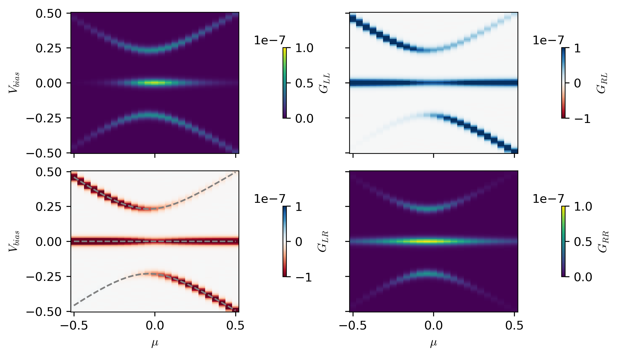
# Calculate the excitation spectra for validating the results
excitation_spectra = []
for _mu in _mus:
    params = parameters.copy()
    params["mu_L"] = _mu + _mu_L
    evals, _ = utils.fermionic_eigsh(f_hamiltonian(**params), parity=parity_operator)
    evals = np.array(evals)
    excitation_spectra.append(
        [
            # transition within a parity sector
            evals[0, :] - evals[0, 0, np.newaxis],
            # transition between parity sectors
            evals[1, :] - evals[0, 0, np.newaxis],
        ]
    )
excitation_spectra = np.array(excitation_spectra)
bound = 1e-7
fig, ax = plt.subplots(figsize=(7, 4), nrows=2, ncols=2, sharex=True, sharey=True)

im2 = ax[1, 0].pcolormesh(
    _mus, bias[:, 1], conductance[1][:, :, 1, 0].T, cmap="RdBu", vmin=-bound, vmax=bound
)
im3 = ax[0, 1].pcolormesh(
    _mus, bias[:, 1], conductance[1][:, :, 0, 1].T, cmap="RdBu", vmin=-bound, vmax=bound
)
im4 = ax[1, 1].pcolormesh(
    _mus, bias[:, 1], np.abs(conductance[1][:, :, 1, 1].T), vmin=0, vmax=bound
)
im1 = ax[0, 0].pcolormesh(
    _mus, bias[:, 1], np.abs(conductance[1][:, :, 0, 0].T), vmin=0, vmax=bound
)

ax[1, 0].plot(_mus, excitation_spectra[:, 0, :2], "--", c="gray")
ax[1, 0].plot(_mus, excitation_spectra[:, 1, :2], "--", c="gray")
ax[1, 0].plot(_mus, -excitation_spectra[:, 0, :2], "--", c="gray")
ax[1, 0].plot(_mus, -excitation_spectra[:, 1, :2], "--", c="gray")

ax[0, 0].set_ylabel(r"$V_{bias}$")
ax[1, 0].set_ylabel(r"$V_{bias}$")

ax[1, 0].set_xlabel(r"$\mu$")
ax[1, 1].set_xlabel(r"$\mu$")

cbar1 = fig.colorbar(im1, ax=ax[0, 0], location="right", shrink=0.5, label=r"$G_{LL}$")
cbar2 = fig.colorbar(im2, ax=ax[1, 0], location="right", shrink=0.5, label=r"$G_{LR}$")
cbar3 = fig.colorbar(im3, ax=ax[0, 1], location="right", shrink=0.5, label=r"$G_{RL}$")
cbar4 = fig.colorbar(im4, ax=ax[1, 1], location="right", shrink=0.5, label=r"$G_{RR}$")